hantverkskod

Introduction

I don’t do much programming in my day job nowadays. It’s still my biggest passion though, so I try to make time for it outside of work. As I’ve gained more experience and had less free time, the circles in the Venn diagram of projects I want to do and projects I can do have drifted so far apart that they no longer overlap (recent observation: ML code generation might change this equation).

Since this is supposed to be a hobby, there’s no point working on projects I don’t want to do.  This means I need to work on projects I can’t do if I want to do anything. That’s the main reason I’m starting a blog about 20 years after blogging was du jour. It will give me a chance to give my projects a little send-off before I abandon them in the wilderness.

Some years ago, I got the idea to write my own implementation of Pixar’s PRMan (photorealistic RenderMan) renderer. At face value, this is clearly an absurd idea. Pixar has a large team of engineers who have been working full time on this for close to 40 years. I’m a single person squeezing in a few hours of programming here and there. That said, as a professional programmer I also know that the last 10% of a project can take 90%, and even that’s probably optimistic. So if you only implement the parts you’re actually interested in, you can get surprisingly far. I’ll go into more detail about what that means for this particular project.

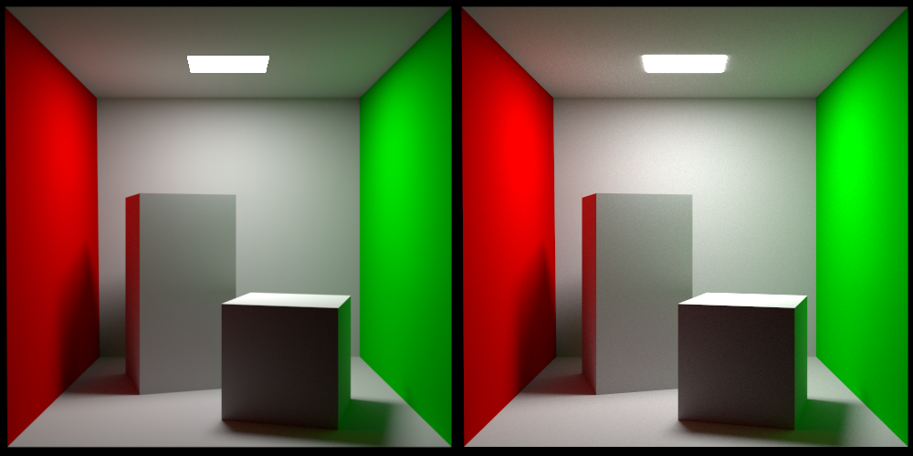
Without further ado, here is the classic Cornell box rendered with PRMan on the left and my own renderer on the right:

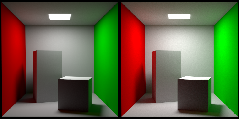
I got this scene from Jan Walter’s site. This is a great resource since it has test scenes rendered by a lot of different renderers for comparison. I’m loading my scene using the ASCII version of the RIB (RenderMan Interface Bytestream) format. Pixar used to make a specification of this format available, but unfortunately they no longer do. I’m not sure why, but my theory is that when they moved from their original rasterization-based REYES renderer (Renders Everything You Ever Saw) to their path-tracing-based RIS renderer (RenderMan Integrator System) they didn’t feel it was worth the effort to keep the specification up to date.

I’m not planning on writing a detailed series of articles on how to implement a path tracer. There are better sources for that, like this, this, this, or your friendly neighborhood LLM. Instead, I want to comment on some things I found interesting while working on this and maybe provide some intuition to help people get started.

The image on the left is rendered with Pixar’s PxrVCM integrator. This is one of the two production-quality integrators they make available, the other one being PxrPathTracer, which is a forward path tracer with next event estimation etc. VCM stands for vertex connection and merging and refers to this article. What VCM does is reformulate photon mapping as a path sampling technique so that it can be incorporated into the multiple importance sampling (MIS) framework.

My own integrator is a straightforward bidirectional path tracer using MIS as well. I might implement the vertex merging path sampling technique eventually, but for now I haven’t bothered with it.

MIS

The framework of MIS was formalized in Eric Veach’s landmark 1997 dissertation, “Robust Monte Carlo Methods for Light Transport Simulation”. Now, this is the Kajiya rendering equation:

This integral can be thought of as integrating the radiance contributions over all possible paths (the “path space”) from x to a light source in the scene. We can approximate this integral by using Monte Carlo integration over a random subset of the path space. The core idea of MIS is that different ways of sampling this path space (a sampling “strategy”) are better than others at dealing with different scene conditions. If we take the example of direct lighting, that is, light coming directly from a light source, the two obvious sampling strategies are:

1. We can randomly trace a ray from x into the scene and return the emitted radiance of any surface we hit. It is also common to use knowledge about the BSDF to send more rays into directions where it has a high value. For this reason this strategy is often referred to as sampling the BSDF.
2. We can randomly select a point on the surfaces we know are emissive and connect it to x. This is referred to as sampling the lights.

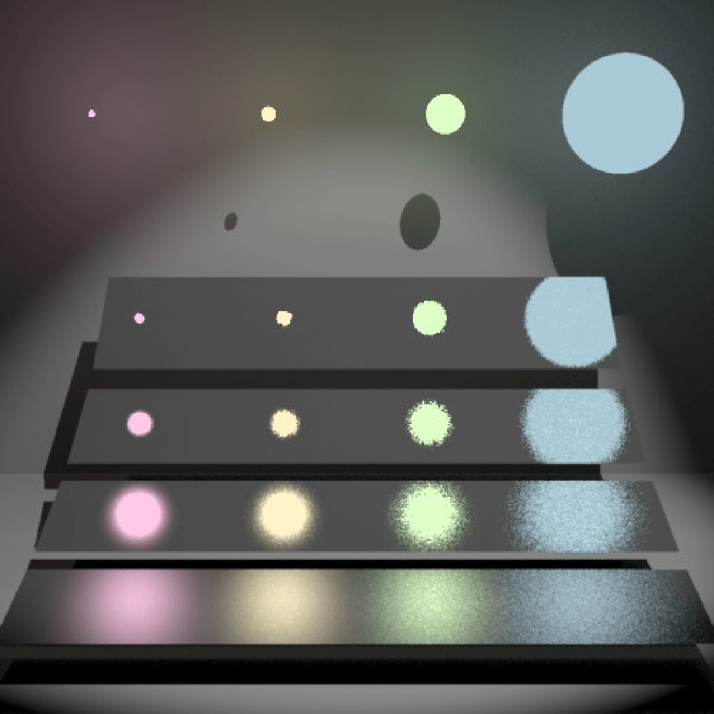
Here’s another illustration showing the results of these two sampling strategies, taken from Veach’s dissertation:

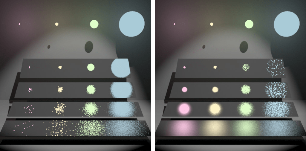
The materials get progressively smoother from top to bottom. Let’s take a look at what’s happening in the top right corner and lower left corner:

• In the top right corner we can see that sampling the BSDF gives much better results than sampling the lights. Since this is a smooth surface, most of the radiance will come from the main direction of reflection, which we’re biasing our samples towards. When we’re sampling the light sources, we’re taking samples from the pink, yellow, and green lights as well, which end up being wasted.
• In the lower left corner we can see that sampling the lights gives much better results than sampling the BSDF. Since this is a rough surface, radiance from all light sources will contribute to the result. These light sources are what we’re taking our samples from. When we’re sampling the BSDF, we’re taking samples from a lot of directions which don’t hit a light source, which end up being wasted.

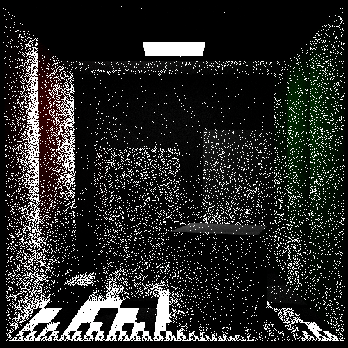
Say we’ve generated a number of samples using these two strategies. Now, what weights should we assign to them to get a low amount of noise everywhere? An initial instinct might be to give them equal weight, but that just leads to noise everywhere:

Veach’s insight is that a provably good way to weight the results of the sampling strategies is something he refers to as the “balance heuristic”:

In this expression:

• $x$ is a sample path (a sequence of vertices connecting the camera to a light source) from the path space generated using some strategy.
• $p_i(x)$ is the probability density of picking this sample using the i:th strategy.
• In the denominator we sum the probability densities of generating this path under all the different strategies we’re using. In the example, that would be both sampling the BSDF and the light sources. This means that we need to be able to take a given path and figure out the probability density of generating it with a given strategy.
• $\hat{w}_i(x)$ is the weight of this sample.

In Veach’s dissertation, there is an extra variable n involved:

This models the scenario where we’re not taking the same number of samples using each strategy (say we’re taking twice as many light samples as BSDF samples).

One final note: we’re free to apply any function we want to the terms in the numerator and denominator and the result will still be unbiased:

A common variant of the balance heuristic is to raise the terms to some power (often two, which empirically is a good choice). This is referred to as the power heuristic. Finally, here are the two strategies combined using the balance heuristic.

Bidirectional path tracing

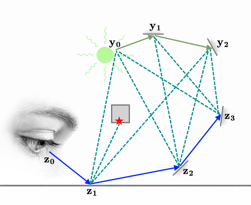
Bidirectional path tracing is a generalization of the idea of the two sampling strategies we introduced in the example above. Instead of just picking a single vertex, we can trace a longer path from one of the light sources. The path starting from the light is usually referred to as the light sub-path, while the path starting from the camera is referred to as the eye sub-path. Now, how do we connect these?

In the standard formulation of the rendering equation, we’re integrating over the solid-angle domain. We can reformulate this as a surface area domain integral instead:

The term $V$ is the visibility function and is defined as either one or zero depending on whether the points $x$ and $y$ can see each other.

Imagine we’re approximating the value of the rendering equation using Monte Carlo integration and we’ve reached the end of the eye sub-path. At this point we decide to switch to integrating over the surface area domain. The surface point ($y_k$) we select to connect to is the one at the end of the randomly generated light sub-path, for which we’ve already computed the probability density and radiance throughput:

This is not a rigorous derivation of bidirectional path tracing, but it is fundamentally correct.

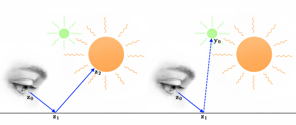
Finally, generating an eye and light sub-path lets us construct a whole family of paths. The dashed lines in this diagram are referred to as shadow rays since they need to take the visibility function $V$ into account.

Putting it all together

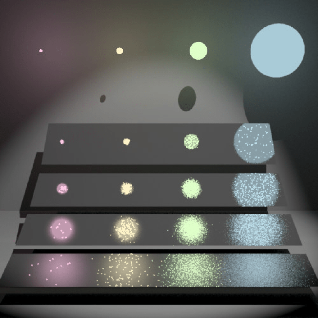
Here is one more illustration of a few different sampling strategies, modulated by MIS weights (balance heuristic) and rendered using my own renderer:

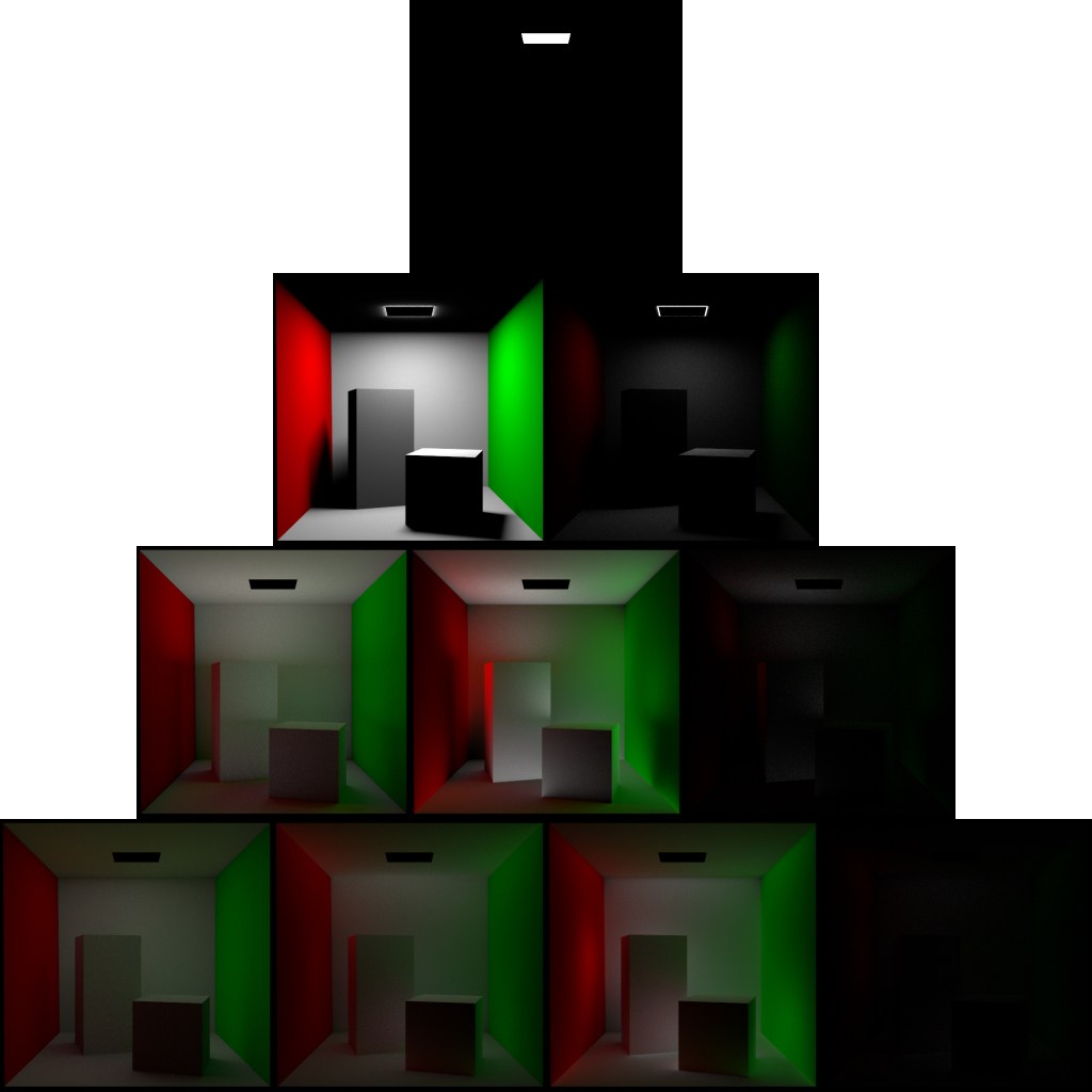
The total number of vertices in the paths increases by one with each row, starting with a single vertex on the first row. The number of light sub-path vertices in each path increases by one with each column, starting at zero. This means the leftmost column corresponds to pure forward path tracing. If we removed the MIS weights, all the entries of each row would be the same except for varying amounts of noise.

A final note, the exposure in the diagram above is increased by one stop per row to make the diagram more legible.

Floating point issues: part one

Path tracing involves a lot of computational geometry, that is, finding the intersection between rays and surfaces etc. If we express our various intersection tests using plain floating point representations of positions and vectors, we get a lot of false positives where rays are incorrectly classified as intersecting with the surfaces they started from.

Two ways of getting around these kinds of issues in the general field of computational geometry are to use predicates or, when possible, an exact representation like rational numbers. Neither of these methods can exactly handle intersection tests between rays and quadrics though.

In practice, what I and other people do is to give the start point of each ray a little nudge (an epsilon) in the direction of the normal of the surface it is starting from. The best way of doing this is to use the approach described by Bruce Dawson here, where floating point numbers are reinterpreted as integers before the epsilon is added. This is the idea behind a “A Fast and Robust Method for Avoiding Self-Intersection” by Carsten Wächter and Nikolaus Binder. Contrary to what the name would have you believe, this is unfortunately not robust. You will still have problems where the nudging pushes the starting point behind surfaces it’s in front of, and choosing a good nudging amount is more of an art than a science.

This is the least satisfying part of working with this project. You know you’re walking around in a field of rakes and you’re just waiting to step on one.

Back to our regular programming

Here again is a comparison between PRMan on the left and my own renderer on the right:

There are two small but obvious differences between the two renders. First, my own render is slightly brighter. I have spent a lot of time trying to figure out why this is without reaching a clear conclusion. In the process of doing so, I have at least found a few things that I do not believe explain it:

• It is not a problem with the tone mapping. The light source can be used to directly compare radiance values. I installed PRMan locally and rendered comparison images with different light settings and the radiance of the light itself came out identical between the two renders in all cases. When displaying to a PNG file sRGB is used as the color space and radiance values exceeding one are clipped.
• It is not the BSDF. The surfaces in the scene are using the Pixar LMDiffuse material which corresponds to an Oren Nayar micro facet distribution. The smoothness is set to one though which reduces it to a pure lambertian model. I have a setting to render a reference image using forward tracing and completely uniform sampling. This produces an identical image to my more sophisticated integrator.
• The RenderMan standard does not specify which color space color values are specified in. I tried interpreting the values as linear instead of sRGB but this leads to a radically different image, so for now I am assuming that color values are indeed specified in sRGB.
• It is not the handling of double sided lights (see below, and thanks to Jon G. for suggesting that this could be the problem). Even with “Sides 2” commented out in the RIB file, the image remains brighter.

If anyone has additional theories as to what the problem could be, I would be happy to hear them.

Second, the shape of the light is different which is less surprising. I am fairly sure PRMan is applying a filter to subtly anti-alias the image and also mimic the presence of the point spread function. If you look at the shape of the light in my render, it might look like I am doing so as well, but the apparent glow around the light is actually due to it being modeled as a double-sided rectangle slightly offset from the roof geometry. The “glow” you are seeing is direct light from the back of the light. For comparison, here is a render from Arnold (which seems to ignore the double sided nature of the light).

As you can see, the shape of the light matches that of my render.

Next time

• Refractions
• Specular lobes
• New rakes
• And more!

A big thank you to my colleagues Jon G., Kyle H., and Tom H. for reviewing this before I posted.