ENHANCE!

Image from Super Troopers (2001), © Fox Searchlight Pictures.

I don’t need to be an expert in everything, but I want to know enough to make well-informed decisions. I have some experience writing both multi-layer perceptrons (MLPs) and attention/transformer-based models (for instance language models) using both PyTorch and TensorFlow, but I hadn’t experimented with convolutional neural networks (CNNs) yet. As the name suggests, CNNs are built around convolutions. These are just filters whose weights are learned during training. The same filters are then applied across the entire input. CNNs feature heavily in modern image processing. NVIDIA’s super-resolution model used CNNs up until DLSS 4.

I was interested in writing my own denoiser. There’s a family of CNNs called U-Nets that are particularly well suited for this (and many other sophisticated tasks). These networks consist of a series of filters that detect features at progressively larger scales (the encoder stage), which are then recombined through another series of filters (the decoder stage). They got their name from the fact that, when you plot the network topology, it forms a U shape (we’ll get to the topology of my own network later on)

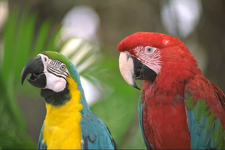
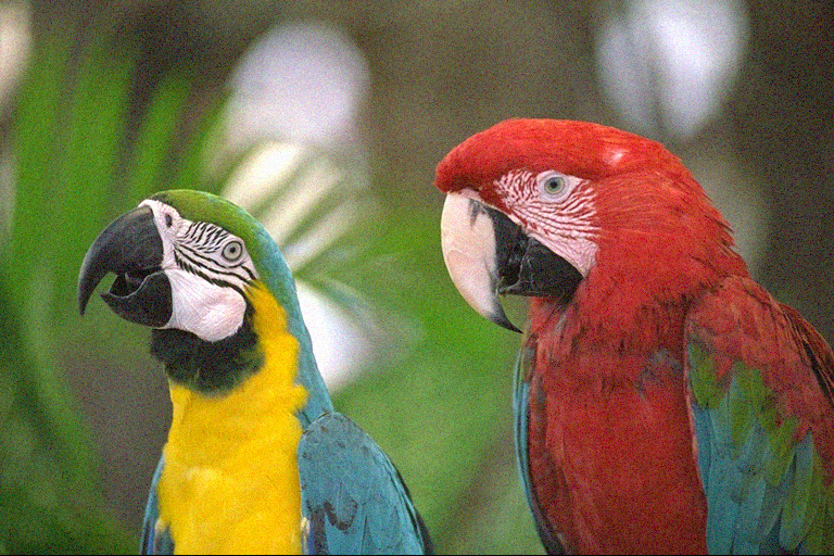
A picture is worth a thousand words, so without further ado, here’s the result of my little project.

This turned out much better than I thought it would, especially considering how little time I spent training it (relatively speaking). Some fine detail gets lost, but overall I’m pleased with the result. (Image from the Kodak Lossless True Color Image Suite)

I used PyTorch with Codex for this project. I’ve worked on a number of PyTorch and TensorFlow projects in the past, and the coding itself isn’t particularly creative, so I was happy to leave it to Codex this time. The interesting part is designing the topology and deciding which training parameters to use.

Training

The first thing I did was run short tests for a fixed amount of time with different hyperparameters on a small set of test images. The things I varied were:

The topology, i.e. the number of layers and channels in the network
The learning rate
The patch size

Like the learning rate, the patch size is not part of the model architecture. The biggest advantage of using smaller patches is that they are computationally cheaper, so for the same amount of training time the model can see a larger variety of inputs. The downside is that each input has less spatial context, meaning the model can’t learn features larger than the patch itself. It also means that a larger fraction of the training pixels are near a patch edge and therefore see artificial padding rather than real neighboring image content.

Once I had a winner, I trained it for much longer (around ten hours) and on a larger dataset. Here is an illustration of the winning topology. Normally these diagrams flow from left to right, but that would make the image too wide for the blog layout. If you lie down and look at your monitor through a mirror, though, you’ll clearly see the U shape. The dimensions in each box is the size of the output after applying the filter.

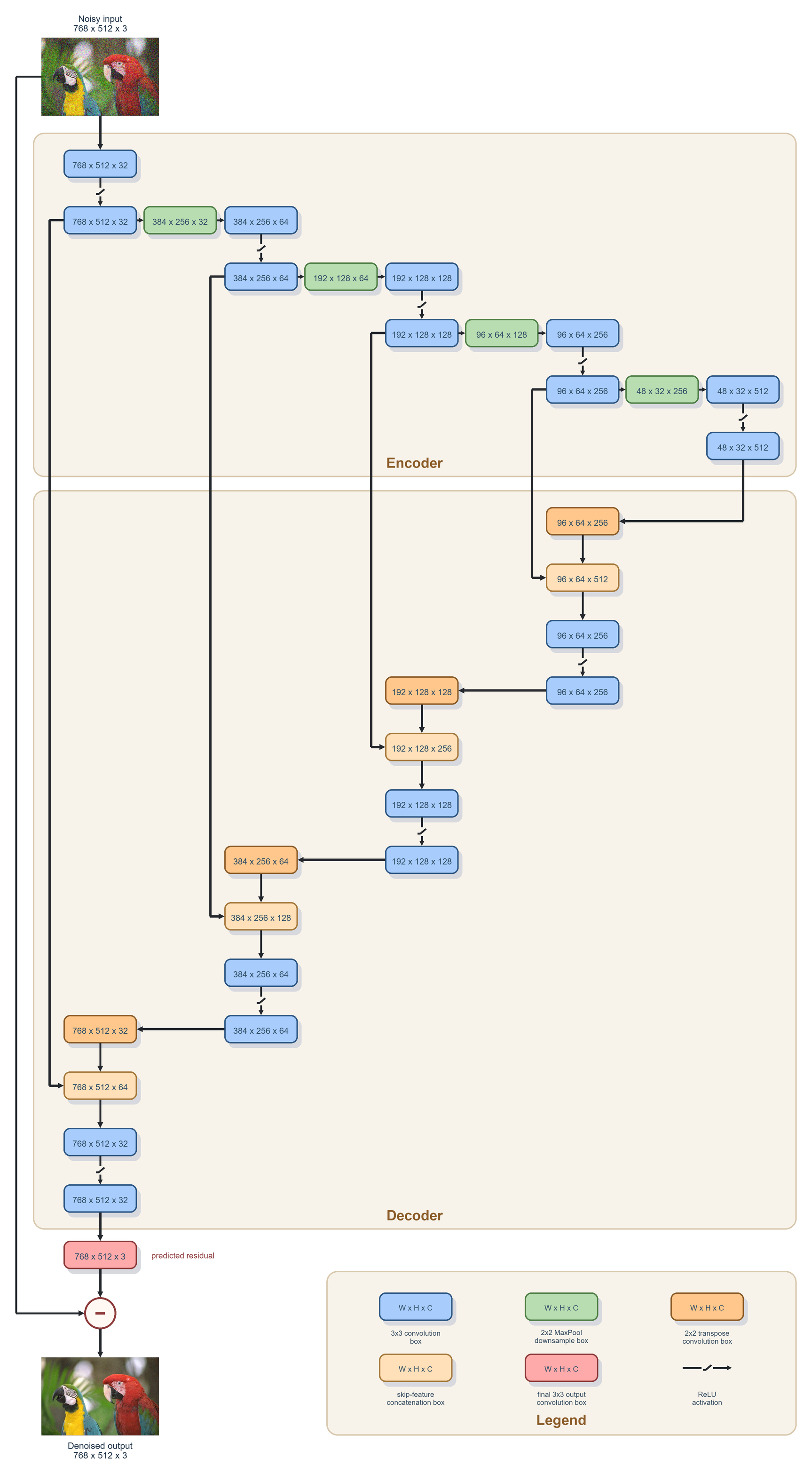
Winning Residual U-Net Topology, Patch size 128 x 128, Learning rate 1e-3

The network doesn’t learn the denoised image directly. Instead, it learns the added noise itself (the residual), which is then subtracted from the source image to produce the denoised image.

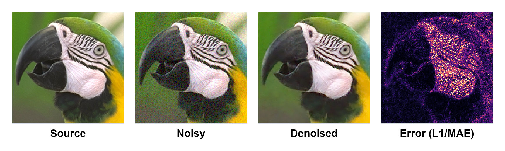
The model operates in linear space and uses mean absolute error as the training metric. This isn’t ideal because it doesn’t take into account how the human eye perceives contrast and color, instead treating each linear RGB channel independently. There are other metrics like LPIPS, FLIP, and MS-SSIM that are more aligned with human perception, but for the first version I wanted to keep things simple. Here is the full source image from above, the noisy version, and the denoised one.

Network DEtails

My preferred way of thinking about convolutions is as one function weighting another. For two functions $f$ and $g$ , the convolution is defined as:

(f * g)(t) = \int_{-\infty}^{\infty}f(\tau)g(t-\tau)d\tau

For discrete signals, this becomes:

(f * g)[n] = \sum_{k = -\infty}^{\infty}f[k]g[n – k]

Another way to think about these operations is as projections. For instance, the coefficients of a Fourier transform are the projections of a function onto a set of orthogonal basis functions using the definition above. That is, projecting a basis function onto itself gives one, while projecting it onto any other basis function gives zero.

The 3 x 3 convolutions operations

These are the blue boxes in the diagram. The text inside them indicates the dimensions of the output after the filter is applied.

Each operation applies $m$ filter kernels $K_m$ of shape $[3 \times 3 \times {C_{in}}]$ to an input patch $X$ of the same shape. Each filter computes an inner product followed by a bias term, producing one output channel per filter:

y_m = \langle K^{(m)}, X \rangle + b_m

where:

$X$ is the local input patch tensor
$K^{(m)}$ is the kernel tensor,
$\langle K^{(m)}, X \rangle$ is the inner product (dot product),
and $b_m$ is the scalar bias for that output channel.

Returning to the projection interpretation, the resulting value indicates how well the input patch matches a given filter. Traditional hand-rolled filters include things like smoothing and sharpening, as well as Sobel operators, which can be used to detect edges. The filters learned by the U-Net do not map cleanly to any of these, but instead represent abstract features that the model found useful during training.

The 2 x 2 MaxPool downsample operations

These are the green boxes in the diagram. There’s not that much to say about them. They take an input and halve the spatial resolution by selecting the maximum value from each $[2 \times 2]$ input region.

The 2 x 2 transpose convolution operations

These are the darker orange boxes in the diagram. This is similar to the $[3 \times 3]$ convolutions above, except that it applies $m$ filter kernels $K_m$ of shape $[2\times 2 \times C_{in}]$ to an input patch $X$ of shape $[C_{in}]$ (i.e. a single element from the input layer). This doubles the spatial resolution while halving the number of channels.

The concatenation operations

These are the lighter orange boxes in the diagram. All they do is concatenate two inputs of shape $[W \times H \times C]$ into an output of shape $[W \times H \times 2C]$ . This is the recombination step I mentioned earlier.

That’s numberwang!

The network I trained is too large to run in real time. Here’s the total parameter count:

Pass	Kernels + Biases	Sum	Running total
3 x 3 convolution	32 x [3 x 3 x 3] + 32	896	896
3 x 3 convolution	32 x [3 x 3 x 32] + 32	9,248	10,144
…	…	…	…
2 x 2 convolution	32 x [2 x 2 x 64] + 32	8,224	7,732,352
3 x 3 convolution	32 x [3 x 3 x 64] + 32	18,464	7,750,816
3 x 3 convolution	32 x [3 x 3 x 32] + 32	9,248	7,760,064
3 x 3 convolution	3 x [3 x 3 x 32] + 3	867	7,760,931

We can (and will) measure the actual cost of applying this filter, but first I want to do a little bit of numberwang (one of my boss’s favorite phrases) to get a rough estimate of what the cost might be.

Computational perspective

Here’s a table of the number of floating point operations (FLOPs) required to process a full UHD 4K image. For simplicity, I’ve skipped the biases, ReLU, and max-pool operations since they are completely dwarfed by the convolutions. The times two is present since we need both a multiply and accumulation (MAC) for each weight of the filter kernel.

Pass	Calculation	FLOPs	Running total
3 x 3 convolution	2 x 2160 x 3840 x 32 x [3 x 3 x 3]	1.43e10	1.43e10
3 x 3 convolution	2 x 2160 x 3840 x 32 x [3 x 3 x 32]	1.53e11	1.67e11
…	…	…	…
3 x 3 convolution	2 x 2160 x 3840 x 32 x [3 x 3 x 32]	1.53e11	3.05e12
3 x 3 convolution	2 x 2160 x 3840 x 3 x [3 x 3 x 32]	1.43e10	3.07e12

I have an Nvidia RTX 5070 with 12 GiB of memory. According to the spec, it has a theoretical throughput of about 30.9 TFLOPS/s for pure FP32 workloads. Nvidia’s number assumes everything is a fused multiply-add (FMA) operation, which maps perfectly to our use case. If (big if) we assume perfect utilization and infinite memory bandwidth, it means we should be able to complete this in something like 3.07 TFLOPS / (30.9 TFLOPS/s) ≈ 100 ms.

Memory perspective

Another way to look at this is to ask what would happen if computation was free and we were limited only by memory bandwidth. Let’s also assume perfect input reuse, so that each value is only read once. In this table I’m also assuming that the ReLU and max-pool operations require a round trip to memory.

Pass	Read	Written	Running R+W
3 x 3 convolution	0.0927 GiB	0.989 GiB	1.08 GiB
ReLU	0.989 GiB	0.989 GiB	3.06 GiB
…	…	…	…
3 x 3 convolution	0.989 GiB	0.0927 GiB	44.3 GiB
subtraction	0.185 GiB	0.0927 GiB	44.6 GiB

My 5070 has a bandwidth of around 626 GiB/s so if we do some more numberwang we land at 44.6 GiB / (626 GiB/s) = 71.2 ms.

Theory will take you only so far

In reality I don’t need to speculate about the runtime cost, I can just measure it. I ran a benchmark over multiple passes, and the median completion time was 277 ms.

What I wrote above, “Let’s also assume perfect input reuse, so that each value is only read once”, is of course wildly optimistic. Each streaming multiprocessor (SM) has 128 CUDA cores, operates on 32-thread warps, and has 128 KiB of L1 cache memory. A compute kernel can explicitly reserve some of this as thread-group shared memory (groupshared in HLSL), accessible to all threads in a thread group, or leave it available for automatic caching of ordinary memory accesses. This is not a lot of memory.

As an illustration, just the weights of the largest filter kernel required to produce one output channel occupy 512 x 3 x 3 x 4 bytes = 18 KiB. Even an implementation making optimal use of shared memory and caching will have to refetch a lot of data, which likely explains much of the discrepancy between our ideal and actual result.

What’s next?

This was a fun project. When the DirectX Compute Graph Compiler becomes available, I’d be interested in trying to optimize the model and get it to run in real time, at least on my 5070.

Another thing I might try before that is using it to denoise the results of my path tracer. This first version only takes RGB as input, but it would be easy to update it to take additional G-buffer channels as inputs, which would help the network identify features.

Finally, I’m also interested in adapting this denoiser for super-resolution. I have some ideas in this space that I want to try.