hantverkskod

I’ve recently been spending more of my time experimenting with various ML algorithms. I’m currently in the process of updating my super resolution project to use attention layers. Before I fully immerse myself in that, I want to wrap up my path tracing project and write a few words about the things I promised to cover in my first post.

New scene, camera one

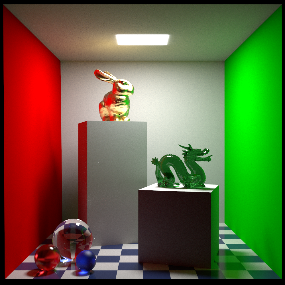
This scene is once again from Jan Walter’s site. For the Cornell box render in my first article, it was relatively straightforward to match the Pixar reference since the BRDF was a pure Lambertian. As I move on to more complicated materials, it gets more difficult to reverse engineer the exact behavior since the documentation only gives hints about how things work behind the scenes. It’s like Plato’s shadows on the wall of the cave. For this reason, I’m going to focus more on qualitative than quantitative differences. Also, I will not try to sweep the errors in my renderer under the rug. These errors are actually some of the most interesting things to talk about. Here’s a render of the new scene from the first camera angle:

Specular reflection

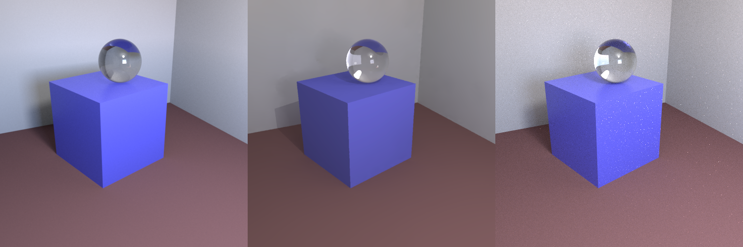
This scene contains specular materials. The blue podium uses the PxrLMPlastic material (these materials have been superseded by a more general model in newer versions of PRMan), which has a specular lobe. The specular lobe is most clearly visible in the faint reflection of the crystal ball on top of the podium.

The material still uses an Oren–Nayar diffuse reflectance model for the diffuse lobe. For the specular lobe, I’m using a Beckmann microfacet distribution (also known as a normal distribution function, or NDF), a Smith shadow-masking term, and a physically accurate Fresnel model rather than the commonly used Schlick approximation.

Let’s talk a bit about how to integrate this dual-lobe material into a bidirectional path tracer with multiple importance sampling (MIS). So far, I’ve not shown any source code in my articles, but for this section, it is helpful to look at how I’ve defined my material interface:

[[nodiscard]] virtual Vec3f operator () (Pos3f const& xx, Vec3f const& w_i, Vec3f const& w_o, Vec3f const& n) const noexcept = 0;
[[nodiscard]] virtual BxdfSample sample(Vec3f const& w_o, Vec3f const& n, Vec3f const& t) const noexcept = 0;
[[nodiscard]] virtual float pdf(Vec3f const& w_i, Vec3f const& w_o, Vec3f const& n) const noexcept = 0;

There are many ways of doing this. Since this was a learning project for me, my focus was on having an intuitive interface, not the most efficient one.

Evaluation

The first of these functions is simply $f_r$ from the rendering equation (the BRDF), with an added normal parameter to orient the integration domain (I don’t support anisotropic materials, as that would have required a surface tangent as well). There’s not that much to say about this part. It just evaluates the specular and diffuse lobes and returns their sum.

Vec3f BxdfPlastic::operator () (Pos3f const& /*xx*/, Vec3f const& w_i, Vec3f const& w_o, Vec3f const& n) const noexcept {
	auto const diffuse = oren_nayar(w_i, w_o, n, Vec3f(m_desc.diffuse_color), m_desc.diffuse_roughness);
	auto const h = normalized(w_i + w_o);
	auto const fresnel_factor = fresnel(dot(h, w_o), 1.f, m_desc.specular_eta);
	auto const specular = beckmann_reflection(w_i, w_o, n, m_desc.specular_color * fresnel_factor, m_desc.specular_roughness);
	return diffuse + specular;
}

(Snake case, east const, K&R braces, auto auto auto, fight me!)

Sampling

The second of these functions draws a random sample in the integration domain and returns it along with its probability density for use in the Monte Carlo integration. One option would be to draw samples on the hemisphere with a uniform density, but this would allocate too many samples in directions where the integrand is likely to be small. Ideally, I’d like to draw samples with a probability density that matches the magnitude of the integrand. Unfortunately, we don’t have easy access to the $L_i$ term of the integrand, so we’ll have to content ourselves with considering the factors we do have access to:

If we use this function as our probability density, it is still difficult to sample analytically. We have to simplify things further to make this feasible. I use the following simplified probability distribution:

The first term is our approximation of the specular lobe using a normalized Ward microfacet distribution, and the second is our approximation of the diffuse lobe using a pure Lambertian microfacet distribution. Both terms can be sampled analytically. To sample their sum, we can first randomly select one of the terms and then sample from it. I hope this is intuitive. I can already tell that this article will be longer than I’d planned, so I don’t want to include a formal proof. The two 0.5 factors are there to normalize the probability density. Here is the C++ implementation:

BxdfSample BxdfPlastic::sample(Vec3f const& w_o, Vec3f const& n, Vec3f const& t) const noexcept {
	auto const b = cross(n, t);
	float x, y, z, pdf;
	if (std::uniform_int_distribution(0, 1)(random_generator()) == 0) {
		std::tie(x, y, z, pdf) = cosine_hemisphere_sample(pdf_min_value);
		auto const w_i = t * x + b * y + n * z;
		return {w_i, pdf * 0.5f + ward_hemisphere_pdf(w_i, w_o, n, m_desc.specular_roughness) * 0.5f};
	} else {
		Vec3f const w_o_l(dot(w_o, t), dot(w_o, b), dot(w_o, n));
		std::tie(x, y, z, pdf) = ward_hemisphere_sample(w_o_l, m_desc.specular_roughness);
		auto const w_i = t * x + b * y + n * z;
		return {w_i, pdf * 0.5f + cosine_hemisphere_pdf(z, pdf_min_value) * 0.5f};
	}
}

Regardless of whether we sample the specular or diffuse lobe, we return the full probability density for the sampled direction. In other words, for a given sampled direction, the returned probability density is the same whichever lobe was selected.

As for pdf_min_value, in a cosine distribution, as sampled directions approach the terminator of the hemisphere, the probability density approaches zero. These densities will be used in the denominator of mathematical expressions. To avoid excessively small values, which could make the expressions blow up, I combine a uniform distribution near the terminator with the normal cosine distribution so that the density never goes below pdf_min_value. The PDF is, of course, still normalized.

PDF

The last of the functions in my interface simply returns the probability density of a given direction.

float BxdfPlastic::pdf(Vec3f const& w_i, Vec3f const& w_o, Vec3f const& n) const noexcept {
	return cosine_hemisphere_pdf(dot(w_i, n), pdf_min_value) * 0.5f + ward_hemisphere_pdf(w_i, w_o, n, m_desc.specular_roughness) * 0.5f;
}

The sampling function could have called this function directly as well, but since we already obtain the PDF of one of the lobes during sampling, the current approach is more efficient.

Transmittance

Another thing that’s new since the previous post is that the scene contains transparent materials, so we also have to consider transmittance. The code for my materials that support transmittance is significantly more complex and too long to include verbatim. Instead, I’ll just comment on a few of the things I found interesting.

Evaluation

When it comes to evaluating the BRDF (or rather, the BSDF), we now have to consider the entire sphere as the integration domain. The first thing this code does is decide whether we have a reflection or transmission event. This is done by checking whether $w_i \cdot n$ and $w_o \cdot n$ have the same sign. This initially felt slightly dodgy since I was afraid that an unusual sample from the statistical microfacet distribution on the surface could make it ambiguous whether the event was reflection or transmission. In other words, there could be two possible microfacets for the same pair of $w_i$ and $w_o$, one leading to reflection and the other to transmission. I’ve mostly managed to convince myself that this is not possible for a single scattering event (see the illustration further down), but I’m still slightly suspicious of this part. We’re combining a statistical model with exact geometric reasoning which doesn’t sit quite right with me. Let’s accept this as true for now, though. 🙂

In the case of a reflection event, things are fairly straightforward. This calculation is identical to the one used for the specular lobe of my plastic materials.

For transmittance events, things are more complicated. There are two things I thought were worth pointing out. First, it is a bit finicky to figure out the orientation of the microfacet we’re passing through. This is the formula for calculating the refraction of a ray:

You can find a derivation of this in section 2.6 of An Introduction to Ray Tracing. Now, for our transmission calculation, we want to do the opposite. We have the refracted and incoming rays, but want to recover the normal, which corresponds to the microfacet orientation. This looked a bit daunting at first, but then I realized that we can rewrite the equation as:

Where $s$ is a scalar. This means:

And since we’re looking for a normalized vector we can write:

We select the sign so that the dot product between $\mathbf{n}$ and $\omega_i$ is negative.

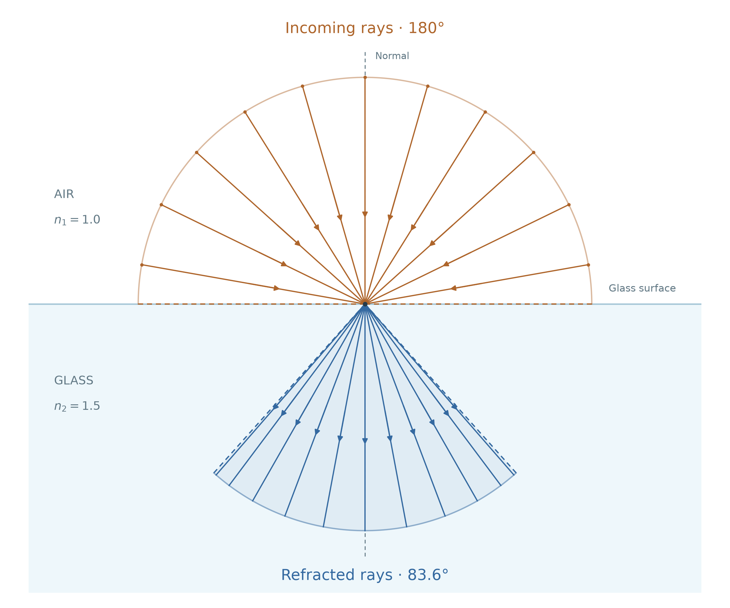
That was long. Now onto the second thing I thought worth pointing out. The radiance of light will be compressed or expanded as it enters an optically denser or rarer material by a factor of $\left(\frac{n_{out}}{n_{in}} \right)^2$.

Sampling

The function that generates a new sample is similar to the one for the plastic material. As with that material, we have two lobes here as well: one for transmission and one for reflection. Unlike with the plastic material, I don’t use equal probabilities to select between the lobes. Instead, I always generate a reflection sample first. I then use the Fresnel factor of the sampled microfacet to decide whether to keep the sample or generate a transmission sample instead. This means we take fewer reflection samples for viewing directions close to normal incidence, where reflection is weaker.

As with the plastic material, the function needs to return the sum of the probability densities for a given direction under the two sampling lobes (reflection and transmission in this case). These lobes are not mutually exclusive but can overlap. Here’s an illustration:

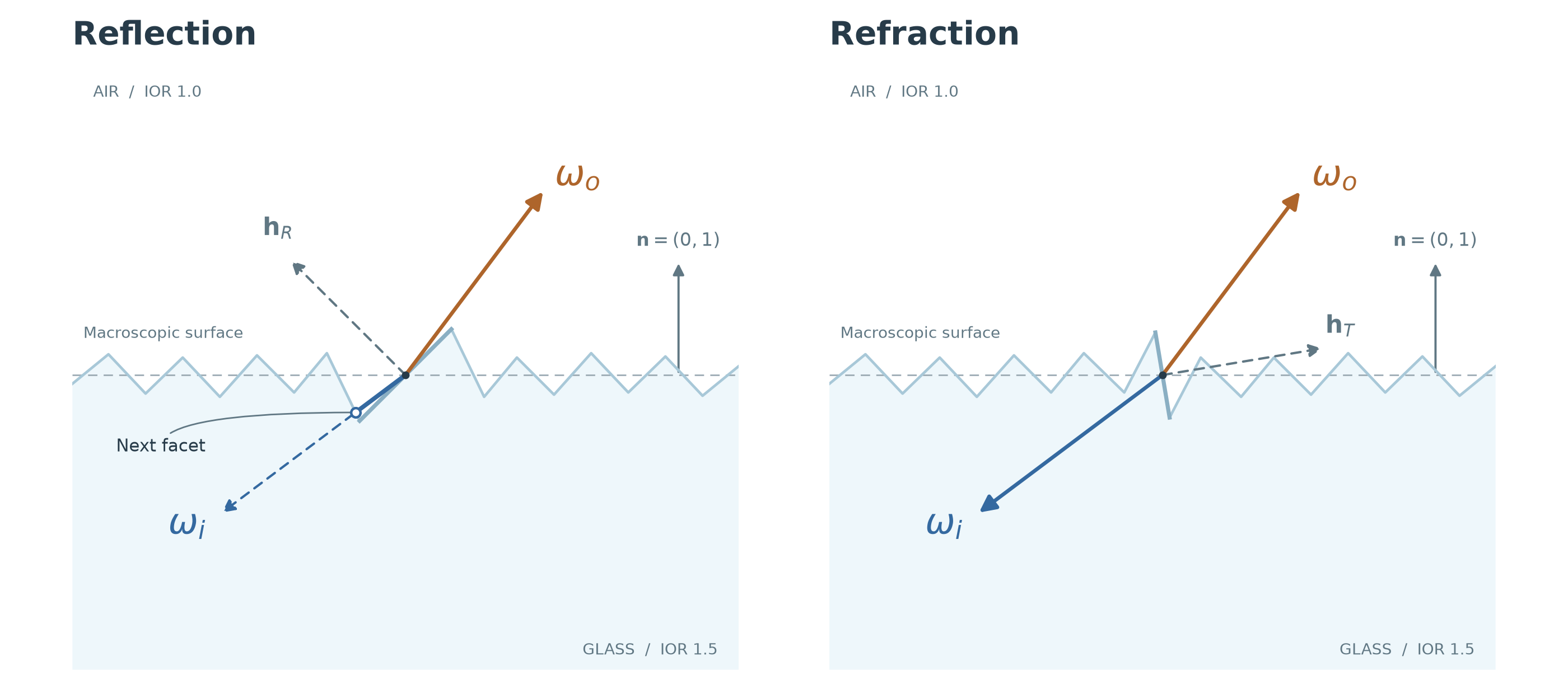
Looking back at the evaluation function, you might remember that we treat all opposing pairs of $\omega_i$ and $\omega_o$ as refractions and all aligned pairs as reflections. This means some samples generated through reflection are treated as transmission (left image above) and vice versa. This won’t result in visual errors. The only thing the sampling function does is generate directions, and the returned value doesn’t carry any information about which lobe was sampled. However, this could slightly reduce sampling efficiency.

PDF

There’s not much to say about this. We just return the sum of the PDF for the reflection and transmission events (same as with the plastic material lobes).

Visual Discrepancies

Let’s have a closer look at some of the differences between my render and those of PRMan and Radiance.

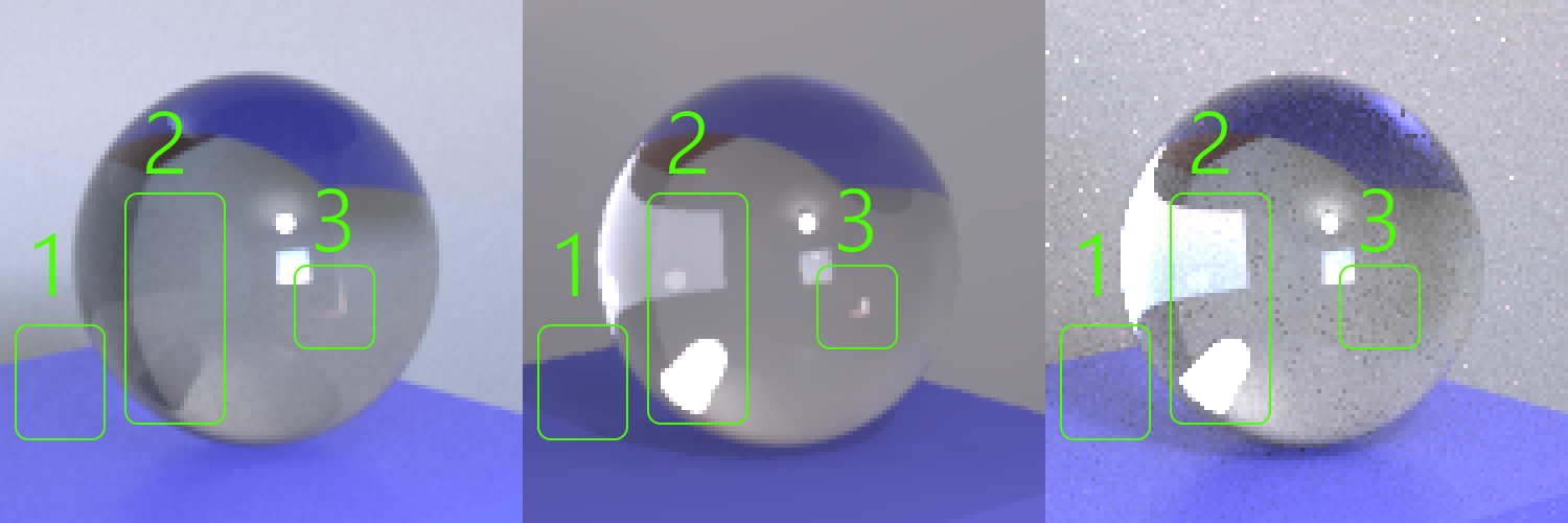
First, there is more noise in my image. I don’t know what Radiance does, but in PRMan, the reduced noise could be due to its use of the VCM integrator, which also incorporates vertex-merging strategies (also known as photon mapping. See my first post about this) that can sample certain light paths more efficiently. The dark noise in my image is due to an overly aggressive variable sampling rate. More on this further down. Looking at the specific issues highlighted in the image above:

1. The PRMan image is missing shadows from the crystal ball. I don’t know why this is. It’s most likely due to an integrator setting.
2. Some refraction contributions are missing from the PRMan render. This is because the VCM integrator in the test scene has a maximum path length of six vertices. The bright areas in my own render receive contributions from paths of length seven (I’m ignoring the VCM integrator’s path-length parameter in the RIB file).
3. It’s not super obvious from the image, but my render is missing a small bright spot. The spot comes from direct sunlight entering through a small glass window, hitting the wall, and making its way through the crystal ball. The full path is something like:
   
   Sun <Light sample>
   Enter glass <Specular Transmittance>
   Exit glass <Specular Transmittance>
   Bounce of wall <Diffuse Reflection>
   Enter glass <Specular Refraction>
   Bounce in glass <Specular Reflection> (possibly need more than one sample)
   Exit glass <Specular Transmittance>
   Eye <Eye>
   
   Even with bidirectional path tracing, there’s an extremely low probability of generating paths like this. The attentive reader will have noticed that the path above has eight vertices. So why does the PRMan VCM integrator, configured with a maximum path length of six vertices, pick it up? I don’t know for sure, but my theory is that the pass that deposits radiance onto surfaces (the photon mapping stage) somehow doesn’t count toward the six-vertex limit, hmm.

New scene, camera two

Metals

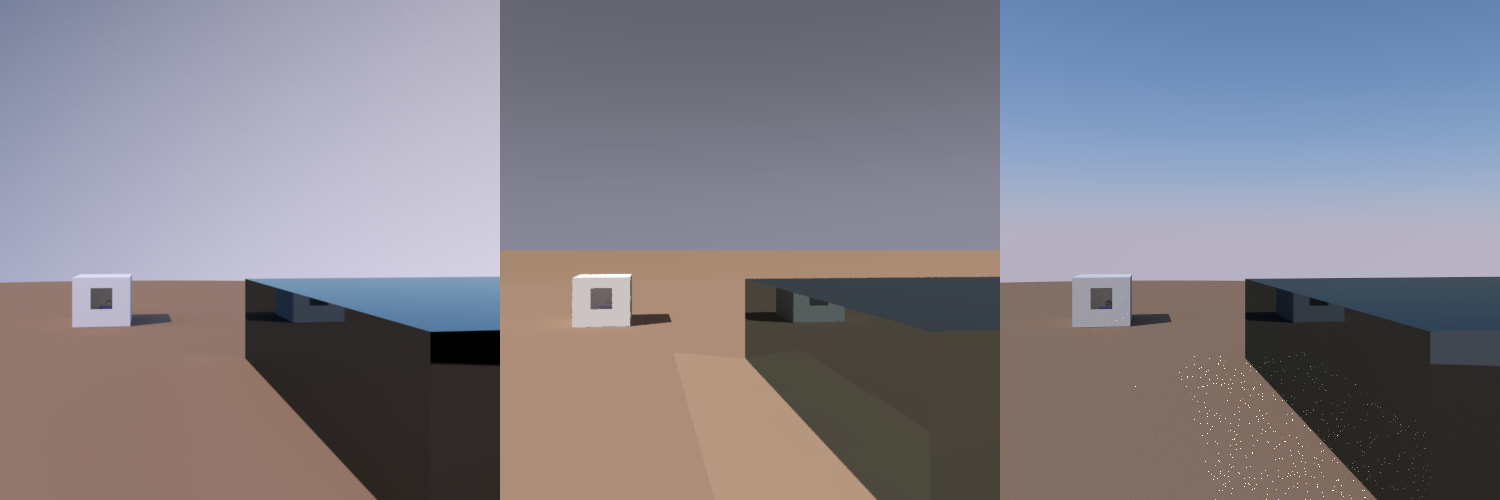
The box on the right uses my implementation of the PxrLMMetal material. There’s not that much to say about this material. It’s much simpler than the plastic or glass materials since there’s only a single specular lobe.

Sky

The sky uses my implementation of PxrEnvDaylight. Like PRMan, my model uses the sky model by Preetham et al., “A Practical Analytical Model for Daylight”. Unlike PRMan, I haven’t modeled the sky as an infinite sphere since doing so would complicate my path-tracing code more than I could justify. Instead, I use a very large sphere. There are two optimizations worth mentioning.

First, the sun (a small disc) and the rest of the sky are treated as two separate light sources, with a higher probability of sampling the sun.

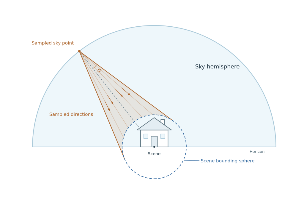
Second, when generating light samples, I don’t sample directions over the entire hemisphere, but only within a small lobe defined by the scene’s bounding sphere at the center of the sky sphere. If I didn’t do this, a lot of the light samples would be wasted since they wouldn’t hit anything. I obviously need to adjust the probability densities to account for this.

Visual Discrepancies

The obvious difference is that the PRMan image is missing the sunlight caustics (unclear why), and those in my render are extremely noisy. Again, this is because the probability of sampling these paths using bidirectional path tracing is very low.

Knowing when to quit!

When you work with a path tracer, you’ll notice that some parts of the image have more noise than others (as in the example with the caustics above). We’d like a way to formalize this observation so that we can allocate more samples to pixels that need them, and fewer to those that have already converged.

Let’s start with a simpler problem. Say we’re rolling dice and want a 95% probability that the average is within 0.1 of the true mean. How many dice do we need to roll?

This is what happens to the distribution of outcomes as one rolls more and more dice:

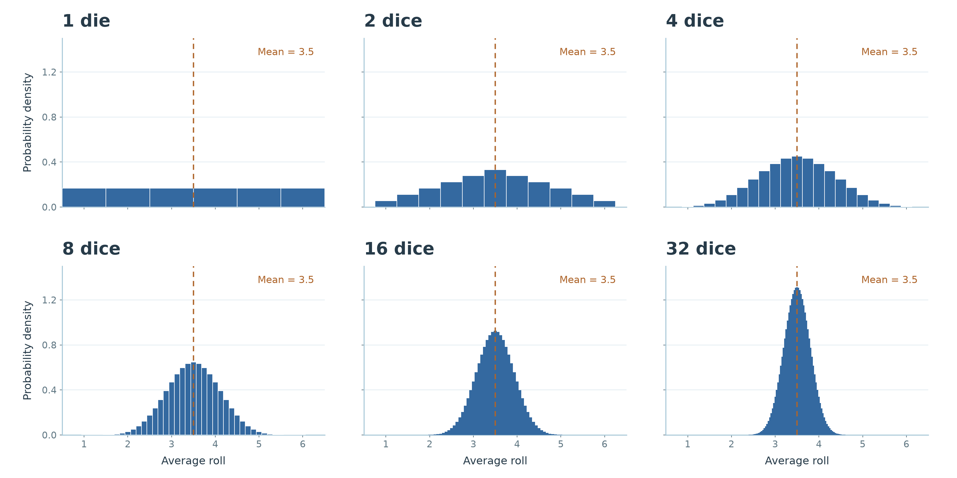
The first thing to notice is that, as we add more dice, the distribution of the average becomes more and more like a normal distribution. This is an illustration of the central limit theorem. From the Wikipedia article:

In probability theory, the central limit theorem (CLT) states that, under appropriate conditions, the distribution of a normalized version of the sample mean converges to a standard normal distribution.

The second thing to notice is that as we add more dice, the distribution becomes increasingly concentrated around the mean. Let’s quantify this. The variance of the average of N dice rolls is:

The value $\sigma_x^2$ is the variance of a single dice roll. If we take the square root of this expression, we get the standard deviation of the sample mean, which is also called the standard error, SE. For a fair six-sided die, $\sigma_x^2$ is exactly $\frac{35}{12}$, so we get:

If we return to the question at the beginning of this section, it can be shown that for a normal distribution, approximately 95% of the values lie within 1.96 standard deviations of the mean. This means we can now solve for the required number of dice rolls $N$:

In other words, if we repeatedly roll 1121 dice, approximately 95% of the time the resulting average will be within 0.1 of the true mean (which is 3.5). This calculation is slightly dodgy since we’re mixing up properties of a continuous normal distribution with a discrete statistical problem, but it is an acceptable approximation for the numbers of dice we actually end up with (I’m fairly sure the exact answer is 1121 as well).

Can we do the same thing for our path-tracing samples, i.e., determine how many samples we need to take so that there’s a 95% probability that our average is within 0.1 of the true mean (which is the radiance we’re looking for)? Each dice roll now corresponds to a sampled path in our path tracer. We can immediately write:

Now we have a problem: unlike in the dice example, we don’t know the true variance of our path samples! We can estimate it using the sample variance, $s^2$, though:

Using this formula, we can approximate the standard deviation of our mean (the standard error) as:

It is important to note that this doesn’t give us an exact bound on the error. What it gives us is a way of estimating the uncertainty of our result, which we can use to decide when we’ve collected enough samples. The inequality above needs to be checked after each sample. This is the programming equivalent of repeatedly asking, “Are we there yet?”. The two constants are obviously arbitrary, and only their ratio matters for the decision on when to break.

For my application, I scale this fraction by the derivative of the transfer function (sRGB in my case), evaluated at the current estimate of the radiance. This is a heatmap showing how many samples were needed to render the image at the top of the article:

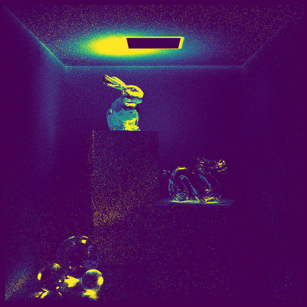
There are two things worth noting. First, I have a configurable cap on the number of samples a pixel can use, and this image is normalized to that range, with yellow indicating the maximum. The fact that we’re seeing yellow in this image indicates that, for these pixels, we didn’t satisfy the statistical stopping condition we’d set up before hitting the ceiling. In other words, these areas are likely to be noisier than the rest of the image.

The second thing to notice is that, again, we’re using a statistical condition to decide when to quit. This image has a million pixels, which means that even in areas of low variance, there are likely to be a few fireflies. You can see one near the top of the podium the golden rabbit is standing on. I actually have a way of removing these fireflies, but I left them in to better illustrate this concept.

Kahan Summation

When you do numerical integration like this, you end up adding up floating-point numbers of very different magnitudes. As the accumulated sum grows, contributions that are small in relation to it will start to get lost if you use ordinary floating-point addition. Even if losing one of these contributions isn’t a problem, with exact arithmetic they could add up to something meaningful, so losing them all can actually be a big deal.

There are a few ways around this. The easiest, and the one I’m using, is the Kahan summation algorithm. What it does is keep track of rounding errors as they accumulate and use that information to correct the final sum. More precisely, I’m using Neumaier’s improved Kahan–Babuška algorithm.

Knowing when to quit?

BrinckMan is currently 100% hand-written. This is probably the last large project I’ll do this way. Let me elaborate.

When I started this article some months ago, the working title was “Killing BrinckMan”. In my first article, written back in February, I mused about AI eventually making it possible for me to take on more projects. This was a form of whistling past the graveyard and didn’t reflect the unease I’d started to feel about where we were heading. What actually happened was that even as the set of projects I could do grew, the set of projects that felt meaningful to me at the time shrank.

In hindsight, I’ve gone through a period of low-intensity grief. I was at my lowest point during my summer vacation. Normally, this is a time when I work on some of my software projects, but I was feeling bummed out by the ever-growing capabilities of AI coding tools. I ended up not touching my computer and instead spent my time tinkering around the house and in the garden (honestly not a terrible outcome 🙂). Over the last couple of months, I’ve slowly started to get out of this funk. What changed was seeing people around me whom I admire using these tools to amplify their abilities and increase their impact, and realizing that there was, of course, mastery to be found here as well.

I see people around me going through the five stages of grief as well. How quickly they get through it seems to depend a lot on how they think about their profession. My current job (mostly) doesn’t require me to write code, but back when I was coding professionally, like many graphics programmers, I found the most joy in beautiful, precise brickwork rather than grand architecture (even though I’ve obviously had to do both). People who identify more with the latter (“architects” – hi Lasse!) seem to move through this process much faster than those who, like me, identify more with the former (“coders”). I don’t think there’s any rushing this, we each need to go through it at our own pace, and I also think it’s important to acknowledge that we are losing something.

I’ve not completely shaken my coder blues, but recently I’m starting to feel more energized again about work in general and my personal projects in particular. I’m going to see what I can do if I lean in even more and really try to master these new tools. I’ve obviously been using agentic coding quite a bit over the last year (the illustrations in this article were generated by AI scripts and things like my Shelby task system are completely AI generated), but I haven’t tried anything truly ambitious with it. I don’t know what that is yet. In my first article, I commented on the absurdity of a single person trying to build a complete PRMan implementation. Maybe that isn’t so crazy anymore. Maybe that’s what I’ll do? Or maybe I’ll pick up one of the many other ambitious projects I’ve started over the years and try to finish it? The only thing I know is that I’m starting to feel somewhat positive about a future of software engineering where I don’t need to lay every single brick myself.

(I’m still going to do a bit of coding by hand to keep my skills sharp, but it will be limited to very specific scenarios where steering the machine takes more effort than doing the work myself, or just for the joy of it in smaller projects.)